(6 * 6) + (12 / 2)[1] 42sqrt(81) * sqrt(9)[1] 27(2 / 3)^(4)[1] 0.1975309log(100)[1] 4.60517exp(4.61)[1] 100.484110^5[1] 1e+05By now, you should have installed R and R Studio (see Chapter 1 for details), and customized R Studio to the Editor theme and font size of your choice (see Chapter 2 for details). If you have not done these things, please do so now before proceeding.
R is a computer language and run-time environment which can be used to do many things, including statistical computing and data visualization. I know, the name is weird. How can it be named after a letter?!
Here’s the deal. R was created by statisticians Ross Ihaka and Robert Gentleman in the early 1990s at the University of Auckland. They developed a coding language to teach introductory statistics based on the syntax of another language at the time called S (programmers loved single-letter names back in the day). Since both their first names (Robert and Ross) started with the letter R, that’s what they chose to call their new language. Seriously.

Importantly, Gentleman and Ihaka spoke with their colleagues who convinced them to release the language for free as part of a philosophy called the Free Software Movement. Under this philosophy, “users have the freedom to run, copy, distribute, study, change and improve the software” (see GNU for more details).
They created a mailing list to discuss all things R in 1994, which quickly became big enough to overwhelm them with many feature requests and bug reports. They then selected a core group of developers who would maintain R. They also enlisted the support of their colleagues Kurt Hornik and Fritz Leisch at the Technical University of Vienna who created the Comprehensive R Archive Network (CRAN), which is a repository of user contributions.
Today, R is a thriving language that receives regular updates by the R Core Team, and boasts about 19,657 user-contributed packages on CRAN. R is free, flexible, powerful, and awesome.

You might have heard of other programs for data analysis, and might be wondering which of these are open-source (meaning free!), and which are proprietary. I list some of the most common statistics programs, and whether they are open source or not in Table 3.1.
| Program/language used for data analysis | Is it Open Source (free) or not? | Company or organization maintaining the program/language |
|---|---|---|
| R | YES | Supported by R Core Team and R Foundation for Statistical Computing |
| Python | YES | Python Software Foundation |
| SAS | NO | SAS Institute |
| SPSS | NO | IBM |
| Stata | NO | StataCorp LLC |
| MATLAB | NO | MathWorks |
| JMP | NO | JMP Statistical Discovery LLC |
| MPlus | NO | Muthén & Muthén |
After looking at the list in Table 3.1, it’s natural to wonder “Why would I ever need to use a proprietary software when free versions exist?” That’s a great question to ask. Personally, I see the main reason people use proprietary software is because they were trained to use a particular program and stuck with it. Whatever works for you! Another reason to use a proprietary software might be because it has functionality which you cannot find in the open-source versions. I have only encountered this case once with a very specific type of analytical approach, but generally speaking there are far more contributors to open-source packages and functions than you will find with proprietary software companies.
This book proudly takes the very opinionated position that R is the best.
The most basic use of R is as a calculator. You can execute calculations in a Script file or in the Console directly. In addition to using any real number, the following symbols and operations can also be used:
| Code | Meaning |
|---|---|
| + | Addition |
| - | Subtraction |
| * | Multiplication |
| / | Division |
| ^ | Exponentiation |
| ( ) | Parentheses/Brackets |
| sqrt() | Square Root |
| log() | Natural Logarithm |
| exp() | Exponential Value |
Just enter the calculation in the Console (or Script File, though the Console is easier for quick calculations) following the appropriate order of operations (PEMDAS). As a matter of style, you want to include a space between arithmetic operators like +,-,*, and/. You also want to add a space after any commas, just like in English. This makes your code more readable.
(6 * 6) + (12 / 2)[1] 42sqrt(81) * sqrt(9)[1] 27(2 / 3)^(4)[1] 0.1975309log(100)[1] 4.60517exp(4.61)[1] 100.484110^5[1] 1e+05As you see, the answer is given following the [1], which just refers to the first position in a vector (to be discussed shortly). Note also that R uses scientific notation, so instead of printing 10^5=1000000, R will print 10^5 = 1e+05. The e here is completely unrelated to the number e (Euler’s number). It just means “10 to the power of.”
You can also easily round a number to a given place using the round() function, in which the first argument is the number or numeric vector to round, and the second argument digits = is the number of decimal places to which you want to round.
x <- log(100)*2.45

print(x)
[1] 11.28267# Let's round this to two decimal places, then one decimal place, and then no decimal places.
round(x, digits = 2)[1] 11.28round(x, digits = 1)[1] 11.3round(x, digits = 0)[1] 11Go ahead and try doing some calculations of your own in the Console! Especially if you’re new to R, the best way to learn R is by doing R over and over again.
A function is a block of code that runs only when it is called. Calling a function just means you are giving the computer a single instruction to do a particular thing. In R, every function comprises a verb followed immediately by parentheses, as in function(). We often have information we want to pass to a function, and these are called arguments. Essentially, the function does the thing we want, and the arguments specify how we want them done, or what information we want the function to use.
Let’s try using the simple print() function to display the phrase “Hello World.”
print("Hello, World!")[1] "Hello, World!"Here we called the print() function and passed it the argument "Hello World!". This resulted in the expected behavior of the value "Hello, World!" being printed (i.e. shown on screen).
Did you know that writing code to print “Hello World” is a programming tradition? It’s often the first thing a student learns to write in a programming language, and comes to us from Bell Laboratories in the 1970s. Learn more here.
Besides using functions to accomplish various tasks, we can also easily create our own functions in R. Creating your own function is often a way to automate a series of tasks to streamline your work. We will tackle this issue later. For now, it will be sufficient to be familiar with the terms function, argument, and call.
Packages are user-written contributions which extend the functionality of R. They typically comprise a set of functions, code, documentation, and occasionally some datasets as well. Packages are stored in R as a library. They only have to installed once, but must be loaded each time you intend to use them. Typically, we only need to use a few packages at a time.
Installing a package typically involves communicating with CRAN, and is easily accomplished using the install.packages() function in which the name of the package you want to install should be placed in the parentheses with quotation marks " ". Go ahead now and give it a shot with the tidyverse package (or set of packages rather) using the following code.
install.packages("tidyverse")If the installation was successful, you should see a message that mentions the package has been successfully unpacked and located somewhere on your computer like this:
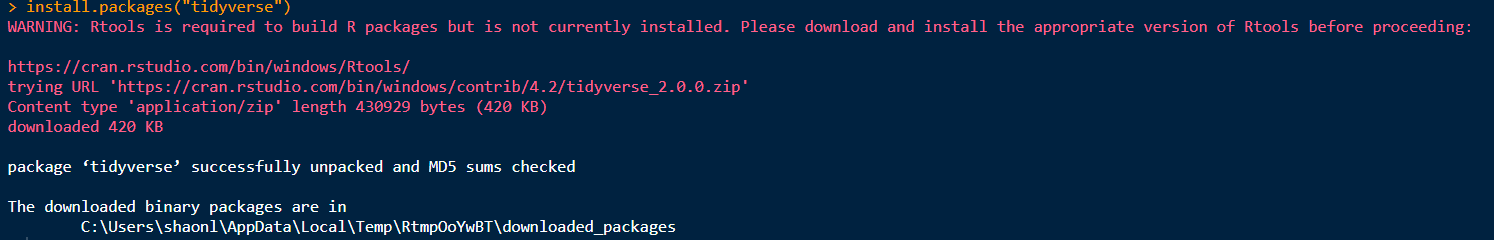
See how it says that the downloaded package is located on my computer? This type of message indicates that there were no problems with the installation. Now, if we want to use this package, it must be explicitly called using the library() function, where the argument is the package name without quotation marks. This is ideally done in a dedicated section called “Load Libraries” or something similar.
# Load Libraries ---------------------------------
library(tidyverse)
Now you know how to install and load packages from CRAN! This is what you will mostly do in R when installing packages, as CRAN packages are all tested and meet certain quality quality standards. To update a package, I find the easiest, cleanest approach is to go to your Output Pane in the bottom right of the screen, go to the Packages tab, and then hit the Update button.
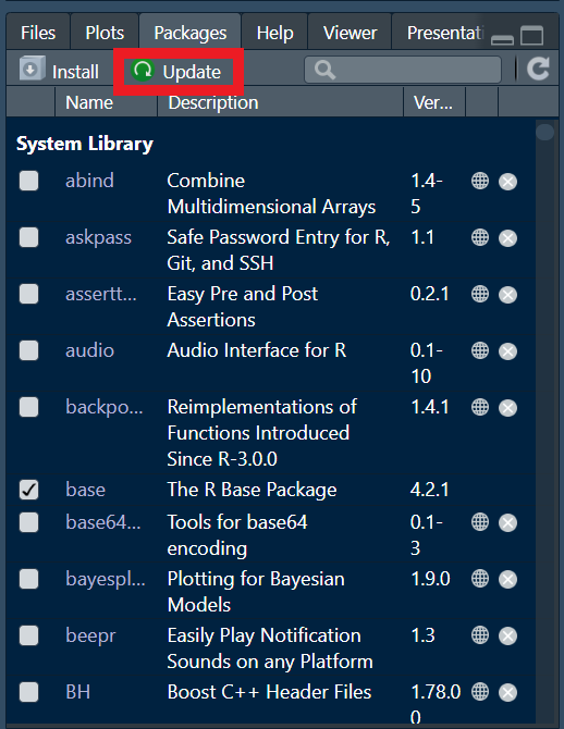
That will bring up a menu which gives you several relevant pieces of information:
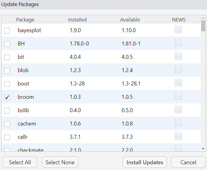
Maybe you don’t want to sit through the updates of EVERY package for which an update is available. This menu allows you to pick and choose the packages you want to update, and then click Install Updates. If you have a specific package you want to update and want to do it quickly, you can use the install.packages() function with the package name to be updated in quotes.
install.packages("bayesplot")Finally, say you want to just update all your packages, and have some time to let R do its thing while you get a coffee, you can just type:
update.packages(ask=FALSE)This will update every package for which an update is available, and the ask=FALSE argument suppresses a prompt from appearing before every package update.
Finally, you may be wondering which packages are essential to install and have ready to go. Typically, you know which packages to use based on a particular task you want to accomplish. Any R script file using packages will always have those listed in the file, and thus you will typically know what packages to install and load.
In R, data are stored as objects. An object is just some data that you have stored. It can be a number, a dataset, a function, or anything else. For example, let’s say we want to perform the following calculations:
((sqrt(81) * sqrt(9)) / log(3.6)) + 6
((sqrt(81) * sqrt(9)) / log(3.6)) - 12
((sqrt(81) * sqrt(9)) / log(3.6)) * (2/3)
We may not want to keep writing ((sqrt(81) * sqrt(9)) / log(3.6)) as it’s cumbersome to work with and to look at. We can streamline the process by assigning ((sqrt(81) * sqrt(9)) / log(3.6)) to a simple name of our choice. Let’s say we assign it to an object called quantity1, the resulting computation would be much easier to write. We can do this by using the assignment operator <- which is comprised of the symbol for less than followed immediately by a minus sign -. So, the code incorporating assignment of the quantity to an object called quantity1 would look like this:
# First, we assign the value to an object called quantity1.
quantity1 <- ((sqrt(81) * sqrt(9)) / log(3.6))

# Then, we can use quantity one in our calculations.
quantity1 + 6
quantity1 - 12
quantity1 * (2/3)
As you’ll notice, the name of the object always comes first, then the assignment operator <-, and finally the value we are assigning to the object.
You can also assign text to an object if you enclose the text in quotes " ".
# Assigning the value Cat to an object called myfavorite.
myfavorite <- "Cat"

# Calling the object directly is the same as calling print(object). It prints the value.
myfavorite
[1] "Cat"Here, I assigned the value "Cat" to an object called myfavorite. I then called that object, and this printed its value. Once you assign a value to an object, it will show up in your Environments Pane on the top-right of your screen. This allows you to keep track of all the objects you have created in your R session, along with their values.

You can also assign the same value to multiple variables using multiple assignment operators <- <- <-. For example, if I want to assign the value male to three names, this is what that would look like.
# Assign multiple variables the value male.
Brendan <- Mark <- Tyrone <- "male"

print(Brendan)
[1] "male"print(Mark)[1] "male"print(Tyrone)[1] "male"If you want to remove an object from your environment, you can use the rm() function with the name of your object in parentheses. For example, if I wanted to remove the object quantity1, I would write rm(quantity1). If you want to remove all objects from your environment, you can run the command rm(list=ls()).
There are some words in R that are reserved for particular tasks. These Reserved Words cannot be used to name an object unless you modify them somehow (e.g. naming an object break1 instead of break). So, don’t ever use these words alone to name an object.
| break | NA |
| else | NaN |
| FALSE | next |
| TRUE | repeat |
| for | return |
| function | while |
| Inf | if |
If you ever need to know how a function works, such as what arguments it takes, you can easily see documentation for it by adding a question mark ? before the function name. For example, if you can’t remember what the rm() function does, or what arguments it takes, you can write ?rm and see the documentation for it. For more complex problems or troubleshooting, you can and should become familiar with Googling the issue, and then seeing the best answer on Stack Overflow in particular. Stack Overflow is one the best places to get answers for R code questions. You should also note that everyone, and I mean absolutely, everyone Googles code issues at some point or another. This is because coding and data science are dynamic fields, and things are often changing. It’s sensible to keep up with how people are solving particular problems by seeing what people are saying on Stack Overflow or other fora.
It’s a good idea to attempt these right away after reading this section while the content is fresh. You can find the answers in Appendix A.
Calculate (89 + 9) / (4*5)^2 and assign the value to the object solution1. Then print solution1.
What is the difference between R and R Studio?
How do you add a comment to a Script file?
What are packages in R, and how do you install them?
Install and load the package rstudioapi.
How do you modify the appearance of R Studio?
Assign the value of 365 to an object called year. Then, create another object called months and assign it the value year * 0.032854884083862.
Create three variables named Cowboys, Giants, and Commanders and assign them all the value "Inferior Team" using multiple assignment operators.
3.3 Comments
You can and should always write comments in your R Script file using a single hash
#. It’s a good idea to use-or=to also clearly break up the Script file into chunks. The easiest and cleanest way to do this is to use Section Headers. On a Windows, you can use Ctrl+Shift+R and on Mac, you can use Cmd+Shift+R to quickly add a section header. You can also go to Code –> Insert Section. Then you can very neatly organize your Script File, like so:It’s a good idea to use comments to explain why you are doing something. For instance, if you are using a specific analytic approach, mention in a comment why you are doing that. I also recommend starting every Script File with the following information on separate commented lines: Title of file, Author, Date, Purpose. Here is an example:
By having clear meta-data for each Script file like this, someone else who reads your code can better understand its purpose, provenance, and format. Additionally, comments on the purpose of a particular line of code can also help you remember why you did something, as it can be easy to forget years later what you had in mind for a particular task.
It can be very useful to know keyboard shortcuts for common tasks. You may want to bookmark this page which lists keyboard shortcuts in R Studio for Mac and Windows.