54/0 [1] Inf-54/0 [1] -Inf0/0 [1] NaNBefore we can dive into data management and cleaning, we need to know what types of data can be stored in R. There are five main types of objects to store data in R. These are summarized in Figure 4.1.
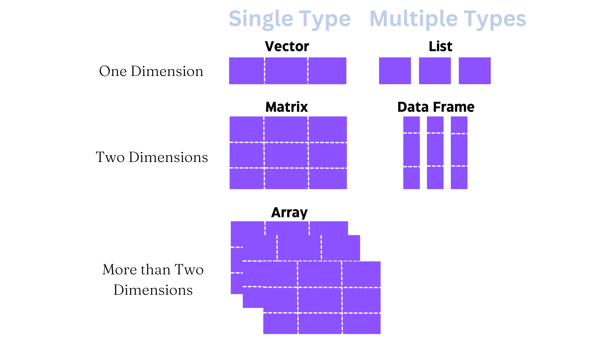
What do we mean by different types of data? Well, data can be many things - text, images, video, recordings, numbers, etc. For our purposes, data will comprise numbers and text. Within these two broad classes, there are five main types of objects used to store data in R, as shown in Figure 4.1. Let’s break each of these down with an emphasis on vectors and dataframes, since we will work with these types most often.
A vector is a sequence of data elements of the same type. In R, there are two types of vectors - atomic vectors and lists. Within the category of atomic vectors, there are six types:
" ").You should note that Doubles and Integers are both numeric vectors, but Doubles are far more common data structures that we typically deal with in social science research. Doubles are quite flexible in that they can be written in decimal, scientific, or hexadecimal form. They also have three unique values: Inf (Infinity), -Inf (Negative Infinity), and NaN (not a number). In practical usage, if you get a value corresponding to any of these three values, something has probably gone wrong! For instance, let’s see what happens when you try to divide certain values by 0 (which is, of course, undefined):
54/0 [1] Inf-54/0 [1] -Inf0/0 [1] NaNIntegers cannot contain fractional values (i.e. no decimals), and are written like Doubles but are followed by an L as in 2L, 3L and so on. Generally, we won’t have to worry about these since we will usually be working with Doubles, Logical, or Character vectors.
Atomic vectors contain elements of the same type. You can always check the type of vector with the typeof() or class() commands. Additionally, you can see the number of elements in a given vector with the length() command.
As mentioned, vectors can comprise strings (pieces of text), integers, or logical values. While they can also comprise a sequence of bytes and complex numbers, we will not discuss these as they are less relevant for our purposes. Let’s start with creating a numeric vector, which can be an integer or double. The most common way to create a vector is to use the concatenate or combine function c() with values in parentheses separated by commas. To create a character vector, you need to surround each element of the vector in quotes " " separated by commas. The paste() function can also be useful in combining vectors.
You can also create a vector comprising a sequence of integers using a colon : between numbers. For instance, a vector containing integers from 30 to 35 assigned to an object obj1 would look like this:
# Create a vector comprising sequential integers from 30 to 35.
obj1 <- 30:35

# Print the values
obj1
[1] 30 31 32 33 34 35Let’s create some more vectors and see how they look.
# Create two numeric vectors.
a <- c(1, 2, 3, 4)
b <- c(5, 6, 7, 8)

# You can do the same thing with a colon instead since the numbers are sequential.
a <- c(1:4)
b <- c(5:8)

# Create a new vector c that combines vectors a and b.
c <- c(a,b)
print(c)
[1] 1 2 3 4 5 6 7 8# Create two character vectors
d <- c("Nirvana", "Alice in Chains")
e <- c("Soundgarden", "Pearl Jam")
# Create a new vector f that combines vectors d and e.
f <- c(d,e)
print(f)[1] "Nirvana" "Alice in Chains" "Soundgarden" "Pearl Jam" # Create three character vectors.
g <- "Four score and seven years ago our fathers brought forth on this continent,"
h <- "a new nation, conceived in Liberty, and dedicated to the"
i <- "proposition that all men are created equal."
# Combine the character vectors using the paste() function.
j <- paste(g,h,i)
print(j)[1] "Four score and seven years ago our fathers brought forth on this continent, a new nation, conceived in Liberty, and dedicated to the proposition that all men are created equal."To extract an element from a vector, we use square brackets [] after the vector name, and write the position of the element(s) we want to extract. We can extract multiple elements by using the concatenate or combine c() function. For instance, if you wanted to extract elements 1, 4, and 5 from a vector called vector1, it would look like this: vector1[c(1,4,5)]. To extract elements in a sequential range, we can use colon : between positions, such as vector1[c(1:5)].
Let’s try an example with a visual summary. First, let’s create a character vector called catbreeds with the values "American Bobtail", "Abyssinian", "Burmese", "Himalayan", and "Manx". We will create the vector with our trusty concatenate or combine c() function. Remember that if you have strings, or pieces of text, these are surrounded by quotes " ". You don’t need quotes if you are creating any of the other vectors mentioned.
# I like one string per line to keep things organized and neat.
catbreeds <- c("American Bobtail",
               "Abyssinian",
               "Burmese",
               "Himalayan",
               "Manx")

# Now I call the vector to see all its elements.
catbreeds
[1] "American Bobtail" "Abyssinian" "Burmese" "Himalayan"
[5] "Manx" Now we have a nice character vector called catbreeds where the different strings (or pieces of text) correspond to different cat breeds. Now, how do we extract or print different elements of the vector? This is summarized in Figure 4.2.
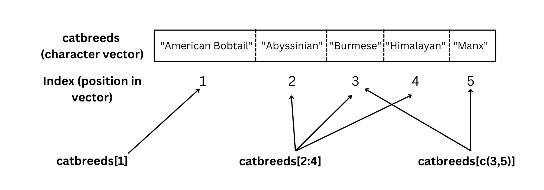
You can see what this looks like in practice below.
# Let's extract "American Bobtail" which is the first element in the vector.
catbreeds[1]
[1] "American Bobtail"# Now let's extract three breeds - Abyssinian, Burmese, and Himalayan.
# These are elements 2, 3, and 4 in the vector.
catbreeds[2:4][1] "Abyssinian" "Burmese" "Himalayan" # What if we want to extract multiple elements that are not sequential?
# Let's do that with Burmese (element 3) and Manx (element 5).
catbreeds[c(3,5)][1] "Burmese" "Manx" You can also extract only positive or only negative integers in a vector by specifying the relevant rule within square brackets after the vector name. For example, let’s create a new vector vectorbeta that comprises only the positive integers of vectoralpha. Then we’ll create another new vector vectorgamma that comprises only the negative integers of vectoralpha.
# Create a numeric vector
vectoralpha <- c(29, 149, 217, -226, 55, 64, -103, -313, 368, 189)

# Create a new vector vectorbeta that takes only positive integers of vectoralpha.
# This code says take all the integers greater than 0 in vectoralpha and assign
# the values to a new vector called vectorbeta.
vectorbeta <- vectoralpha[vectoralpha > 0]
print(vectorbeta)
[1] 29 149 217 55 64 368 189# Create a new vector vectorgamma that takes only the negative integers of vectoralpha.
# This code says take all the integers less than 0 in vectoralpha and assign
# the values to a new vector called vectorgamma.
vectorgamma <- vectoralpha[vectoralpha < 0]
print(vectorgamma)[1] -226 -103 -313In a numeric vector, you can perform a number of operations such as finding the mean mean(), median median(), minimum min(), and maximum max().
# Create a numeric vector

vectoralpha <- c(29, 149, 217, -226, 55, 64, -103, -313, 368, 189)

# Find the minimum and maximum values in the vector.

min(vectoralpha)
[1] -313max(vectoralpha)[1] 368# Find the mean and median of the vector.
mean(vectoralpha)[1] 42.9median(vectoralpha)[1] 59.5You can also perform arithmetic operations on vectors. Let’s create a couple of vectors and illustrate the four basic arithmetic operations. Each operation is performed element-by-element. This means that if both vectors are the same length (same number of elements), the operation will be conducted on the first element of both vectors, then the second element of both vectors, and so on. For example, in vectors a1 and b1 below, addition would involve the following steps: 1 + 2, 3 + 1, and 6 + 4 since these number comprise the first, second, and third elements of each vector, respectively.
# Create two vectors.
a1 <- c(1, 3, 6)
b1 <- c(2, 1, 4)

# Vector Addition
a1 + b1
[1] 3 4 10# Vector Subtraction
a1 - b1[1] -1 2 2# Vector Multiplication
a1 * b1[1] 2 3 24# Vector Division
a1 / b1[1] 0.5 3.0 1.5What happens if the vectors are of different lengths? In such cases, R employs a process called Vector Recycling which takes the elements of the shorter vector and repeats them with elements of the longer vector. R will also give you a warning message to alert you to the different vectors lengths. Let’s look at an example.
# Create a vector of length 4.
c1 <- c(1, 2, 3, 4)

# Create another vector of length 2.
d1 <- c(1, 2)

# Let's look at vector recycling in action when we multiply the vectors.
e1 <- c1 * d1

e1
[1] 1 4 3 8Let’s see how that worked visually in Figure 4.3.
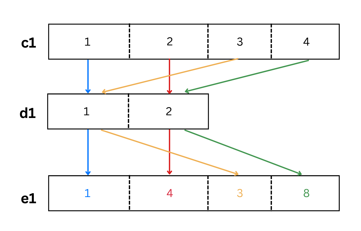
As we see from the colored arrows in Figure 4.3, the elements of the shorter vector d1 were recycled when multiplied by vector c1.

Try creating your own vector and extracting the elements. Once you feel like you’ve got it, only then move on to Matrices. Try creating a numeric vector as well, and extracting its elements using the techniques illustrated above.
A matrix is a two-dimensional vector (i.e. rows and columns.) Matrices are homogeneous data structures in that all elements must be of the same type (e.g. logical, character, numeric) and same length.
You can create a matrix from vectors using the rbind() function to combine rows of data, and using the cbind() function to combine columns of data.
# Let's create three vectors of the same type (numeric) and length (3).

a <- c(.94, .92, .95)
b <- c(.25, .56, .82)
c <- c(.65, .45, .37)

# Then, let's combine the vectors with the rbind() function to combine rows.
d <- rbind(a, b, c)

# Let's combine the vectors with the cbind() function to combine columns.
e <- cbind(a, b, c)

# Now let's print both combined vectors to compare them.
print(d)
[,1] [,2] [,3]
a 0.94 0.92 0.95
b 0.25 0.56 0.82
c 0.65 0.45 0.37print(e) a b c
[1,] 0.94 0.25 0.65
[2,] 0.92 0.56 0.45
[3,] 0.95 0.82 0.37You can also create a matrix using the matrix() function in which the main arguments are the data vector, the number of rows, and the number of columns. Here is a simple matrix with the numbers 1:9 spread over three rows and three columns:
matrix(1:9, nrow = 3, ncol = 3) [,1] [,2] [,3]
[1,] 1 4 7
[2,] 2 5 8
[3,] 3 6 9Do you see the difference between vector d and vector e? In combined vector d, each of the constituent vectors forms a single row. In combined vector e, each of the constituent vectors forms a single column.
You can also change the names of the rows and columns of the matrix using the rownames() and colnames() functions. Let’s try using the matrix() function to input a correlation matrix into R. A correlation matrix is a type of matrix which displays correlation coefficients between variables. A correlation coefficient is a measure of the strength of a linear relationship between two variables on a scale from -1 to 1. A value of 1 indicates a perfect positive correlation, and a value of -1 indicates a perfect negative correlation. A value of 0 indicates no correlation at all between the variables.
There are many types of correlation coefficients, but typically Pearson’s r is used. When you look at a correlation matrix, you will notice that 1s are on the diagonal, because a variable is always perfectly positively correlated with itself. The upper triangle (above the diagonal) is a mirror image of the bottom triangle (below the diagonal), so you only need to focus on one. Personally, I like focusing on the lower triangle, but it doesn’t matter.
Imagine a study on exam performance and study habits with the following variables:
Now let us examine the correlation matrix of the variables of this hypothetical study illustrated in Figure 4.4.
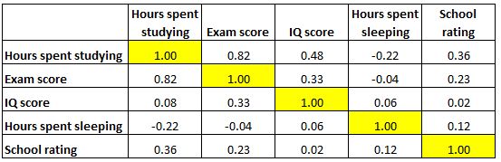
It looks like there is a strong correlation (r = 0.82) between hours spent studying and exam score, which makes sense. We also have smaller correlations between IQ and exam score (r = 0.33) and school rating and exam score (r = 0.23). All other correlations with exam score are negligible. Let’s now input this correlation matrix into R.
# Input correlations

corrs <- c(1.00, 0.82, 0.08, -0.22, 0.36, 0.82,
           1.00, 0.33, -0.04, 0.23, 0.48, 0.33,
           1.00, 0.06, 0.02, -0.22, -0.04, 0.06,
           1.00, 0.12, 0.36, 0.23, 0.02, 0.12,
           1.00)

# Use matrix() function and specify appropriate rows and columns

corrmat1 <- matrix(corrs, nrow = 5, ncol = 5)

# Rename rows and columns

colnames(corrmat1) <- c("Hours studying",
                        "Exam Score",
                        "IQ Score",
                        "Hours sleeping",
                        "School rating")

rownames(corrmat1) <- c("Hours studying",
                        "Exam Score",
                        "IQ Score",
                        "Hours sleeping",
                        "School rating")

print(corrmat1)
Hours studying Exam Score IQ Score Hours sleeping School rating
Hours studying 1.00 0.82 0.48 -0.22 0.36
Exam Score 0.82 1.00 0.33 -0.04 0.23
IQ Score 0.08 0.33 1.00 0.06 0.02
Hours sleeping -0.22 -0.04 0.06 1.00 0.12
School rating 0.36 0.23 0.02 0.12 1.00To retrieve an element of a matrix, write the matrix name, followed by square brackets in which the first argument is the row and the second is the column that you want. For example, if we want to retrieve the correlation between Exam Score and Hours spent studying, we can write the matrix name corrmat1 followed by (row) 2 and (column) 1:
corrmat1[2,1][1] 0.82This retrieves the corresponding correlation of 0.82. Finally, let’s say you want to see the values for an entire column or an entire row. In this case, simply leave the row or column argument blank, but don’t forget the comma ,:
# See the values for column 3 only
corrmat1[, 3]
Hours studying Exam Score IQ Score Hours sleeping School rating
0.48 0.33 1.00 0.06 0.02 # See the values for row 4 only
corrmat1[4, ] Hours studying Exam Score IQ Score Hours sleeping School rating
-0.22 -0.04 0.06 1.00 0.12 
A dataframe is the most common type of data structure we typically deal with in the social sciences. It is a two-dimensional labelled list of vectors, and can have columns of multiple data types. A dataframe’s vectors must be of the same length, which gives dataframes a rectangular structure. A dataframe has rownames() and colnames() just like matrices and lists. The variable names in a dataframe must be different from one another, meaning that the two variables cannot have the exact same name.
If you want to explore R’s built-in dataframes to test out functions and analyses, you can run the data() command to see a list of dataframes.
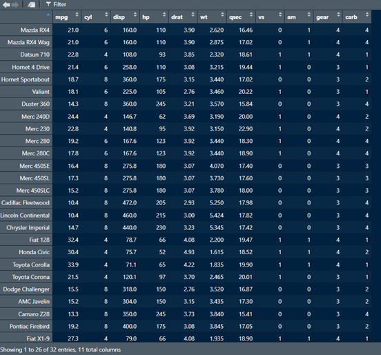
data()Let’s go ahead and use the built-in dataframe mtcars by assigning it to an object called df1 (dataframe 1). Then, let’s look at the dataframe. If you want to have a very quick preview of the first six rows of the dataframe, call the head() function with the name of the dataframe as the argument, and similarly the last six rows of the dataframe can be previewed using the tail() function with the name of the dataframe as the argument.
The head() and tail() functions are useful when you have a very large dataset and cannot feasibly examine the whole thing. However, I find the View() function far more useful. This actually pulls up the entire dataframe in a separate tab.
# Assign the built-in mtcars dataframe to an object called df1.
df1 <- mtcars

# Examine the first six rows of the dataframe.
head(df1)
mpg cyl disp hp drat wt qsec vs am gear carb
Mazda RX4 21.0 6 160 110 3.90 2.620 16.46 0 1 4 4
Mazda RX4 Wag 21.0 6 160 110 3.90 2.875 17.02 0 1 4 4
Datsun 710 22.8 4 108 93 3.85 2.320 18.61 1 1 4 1
Hornet 4 Drive 21.4 6 258 110 3.08 3.215 19.44 1 0 3 1
Hornet Sportabout 18.7 8 360 175 3.15 3.440 17.02 0 0 3 2
Valiant 18.1 6 225 105 2.76 3.460 20.22 1 0 3 1# Examine the last six rows of the dataframe.
tail(df1) mpg cyl disp hp drat wt qsec vs am gear carb
Porsche 914-2 26.0 4 120.3 91 4.43 2.140 16.7 0 1 5 2
Lotus Europa 30.4 4 95.1 113 3.77 1.513 16.9 1 1 5 2
Ford Pantera L 15.8 8 351.0 264 4.22 3.170 14.5 0 1 5 4
Ferrari Dino 19.7 6 145.0 175 3.62 2.770 15.5 0 1 5 6
Maserati Bora 15.0 8 301.0 335 3.54 3.570 14.6 0 1 5 8
Volvo 142E 21.4 4 121.0 109 4.11 2.780 18.6 1 1 4 2# Have a much more detailed look at the dataframe.
View(df1) You can also click the little dataframe icon next to the dataframe in your Environment tab to view the dataframe.
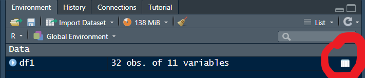
Whether you use the View() function or click the little icon, R will open another tab with the dataframe, and will look something like this:
If we want to know the dimensions of the dataframe (i.e., the number of rows and columns), we can run the dim() function with the name of the dataframe as the argument. This will produce two values - the first indicates the number of rows, and the second indicates the number of columns.
# See the dimensions (number of rows and columns) of a dataframe with dim().
dim(df1)
[1] 32 11If we just wanted to see the number of rows, we can do so using the nrow() function. Similarly, we can see the number of columns using the ncol() function.
# See the number of rows in a dataframe
nrow(df1)
[1] 32# See the number of columns in a dataframe
ncol(df1) [1] 11Another very useful function is str() gives you a quick overview of the type of variables and some of their values in the dataframe. You can get this information using the View() function, which I tend to prefer, but if you want to quickly examine the structure of multiple dataframes, for instance, you can use the str() function.
# See the structure of the dataframe
str(df1)
'data.frame': 32 obs. of 11 variables:
$ mpg : num 21 21 22.8 21.4 18.7 18.1 14.3 24.4 22.8 19.2 ...
$ cyl : num 6 6 4 6 8 6 8 4 4 6 ...
$ disp: num 160 160 108 258 360 ...
$ hp : num 110 110 93 110 175 105 245 62 95 123 ...
$ drat: num 3.9 3.9 3.85 3.08 3.15 2.76 3.21 3.69 3.92 3.92 ...
$ wt : num 2.62 2.88 2.32 3.21 3.44 ...
$ qsec: num 16.5 17 18.6 19.4 17 ...
$ vs : num 0 0 1 1 0 1 0 1 1 1 ...
$ am : num 1 1 1 0 0 0 0 0 0 0 ...
$ gear: num 4 4 4 3 3 3 3 4 4 4 ...
$ carb: num 4 4 1 1 2 1 4 2 2 4 ...Notice how the dataframe comprises rows and columns, where the rows are names of cars and the columns are different attributes of those cars, such as miles per gallon, number of cylinders, displacement weight, and others. To retrieve a particular column in the dataframe, use the dollar sign operator $ after the name of the dataframe, followed by the column name. For instance, if you want to know the mean miles per gallon across all the cars, we can use the mean() function in the following manner:
# Get the mean of the mpg variable in the df1 dataframe.
mean(df1$mpg)
[1] 20.09062From the mean() function used above, we see that across all the cars in the dataframe, the average fuel efficiency is about 20 miles per gallon.
In general, you will use the format dfname$variable to access or refer to any specific variable or column of a dataframe. You can also add a new variable to the dataframe using the same format. For example, if we wanted to add a new column to our dataset df1 in which we take the existing column qsec (the number of seconds it takes the car to travel one-fourth of a mile) and multiply this by four, to get an estimate of how long it takes the car to travel one mile, we can accomplish this with the following code.
# Create new variable in df1 called qsec2 which takes the existing variable
# qsec and multiplies it by four.
df1$qsec2 <- df1$qsec*4

# The mean of qsec2 is predictably four times the mean of qsec.
mean(df1$qsec)
[1] 17.84875mean(df1$qsec2)[1] 71.395To get a quantitative summary of numeric variables in a dataframe, we can use the summary() function to obtain the minimum value, 25th percentile, median, 75th percentile, and maximum value. Let’s try that with the weight wt variable. Then, we’ll obtain the information for multiple variables in the dataframe using square brackets [], the concatenation operator c(), and single apostrophes ' ' around the variable names.
# Summary statistics for only the weight variable
summary(df1$wt)
Min. 1st Qu. Median Mean 3rd Qu. Max.
1.513 2.581 3.325 3.217 3.610 5.424 # Summary statistics for multiple variables
summary(df1[c('mpg','wt', 'qsec')]) mpg wt qsec
Min. :10.40 Min. :1.513 Min. :14.50
1st Qu.:15.43 1st Qu.:2.581 1st Qu.:16.89
Median :19.20 Median :3.325 Median :17.71
Mean :20.09 Mean :3.217 Mean :17.85
3rd Qu.:22.80 3rd Qu.:3.610 3rd Qu.:18.90
Max. :33.90 Max. :5.424 Max. :22.90
While dataframes can contain data of different types (heterogeneous data), lists are even more flexible at doing this. A list is like a collection of different things that don’t have to play by the rules of a dataframe. Recall that though dataframes can contain heterogeneous data, the elements of a dataframe are subject to a few restrictions such as a) they have to be a labelled list of vectors, b) they have to be the same length, and c) the variables must not have the exact same name.
List elements don’t have such restrictions, and you can think of them as collections of different stuff. For example, you can put the contents of a function, a dataframe, a piece of text, numbers, etc in a list. Let’s look at an example of a list called stuff. We will create this list using the list() function and assigning a bunch of random stuff to it. You can even put lists in a list! That’s pretty meta! You can then View() the list to examine its contents.
# Create a list called stuff comprising various random things, including another list.
stuff <- list(catbreed = "manx",
              data = mtcars,
              Euler = 2.71828,
              logical = c(TRUE, FALSE, TRUE, NA),
              random = list(alphabet = letters,
                            greeting = "Hello, World",
                            number = pi
                            )
              )
Once you View() the list, it will show you the contents as in Figure 4.5.
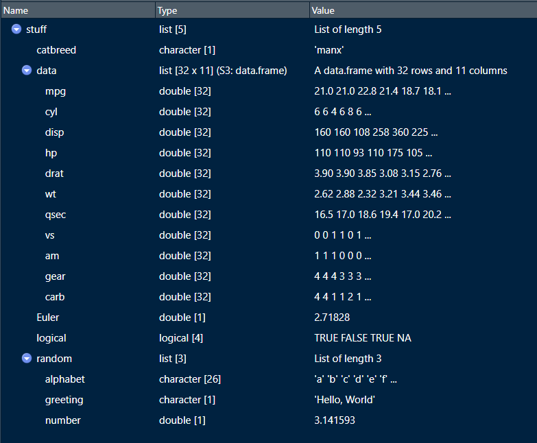
You can see that our list has a string (“Manx”), a dataframe (mtcars), a number (Euler), a logical vector (logical), and another list with three elements of its own (random). Lists are so flexible!
You can extract elements of a list with the dollar sign operator $ if you know the name of the element, or using double square brackets [[ ]] if you know the position of the element. You can also use single square brackets [ ] which will give you a little more information than double square brackets, such as the name of the element.
# Extract elements of a list by name using dollar sign operator.
stuff$Euler
[1] 2.71828# Extract elements of a list by using double square brackets.
stuff[[3]][1] 2.71828# Extract elements of a list by using single square brackets.
stuff[3]$Euler
[1] 2.71828As you see, using single brackets [ ] to extract an element from a list gives you the element name Euler as well as the value 2.71828, as opposed to only the value 2.71828 provided by the double square brackets [[ ]]. In general, if you have a collection of stuff, create a list for easy reference.
Though we will not work with Arrays much, it is worthwhile to know a thing or two about them. Recall that matrices and dataframes are two-dimensional data structures. An array goes beyond two dimensions, and can hold n-dimensional data, but the data have to be of the same type. I think arrays are easiest to understand when thinking about a collection of multiple matrices.
For example, let’s say we have two vectors of different lengths. One vector has three elements, while the other has six elements.
# Create two vectors of different lengths (three and six).
vector1 <- c(1,3,4)
vector2 <- c(32, 4, 7, 19, 23, 43)
Now, let’s create an array where we first create a matrix of three rows and three columns based on our vectors, and then duplicate this matrix four times. We can accomplish this using the array() function where the first argument will comprise our vectors, and the argument dim (or dimension) takes the row numbers, column numbers, and number of matrices we want. So if we want three rows, three columns, and four matrices, the values would be dim = c(3, 3, 4).
# Use previous vectors to create array of four 3x3 matrices.
array1 <- array(c(vector1, vector2),
                dim = c(3, 3, 4)
                )

print(array1)
, , 1
[,1] [,2] [,3]
[1,] 1 32 19
[2,] 3 4 23
[3,] 4 7 43
, , 2
[,1] [,2] [,3]
[1,] 1 32 19
[2,] 3 4 23
[3,] 4 7 43
, , 3
[,1] [,2] [,3]
[1,] 1 32 19
[2,] 3 4 23
[3,] 4 7 43
, , 4
[,1] [,2] [,3]
[1,] 1 32 19
[2,] 3 4 23
[3,] 4 7 43See how we now have four versions of the matrix we requested based on our two vectors? If we want to name our rows, columns and matrices, we can create vectors for those and then feed them into the dimnames (dimension names) argument of array(). The dimnames argument only takes lists, so we’ll assign our name vectors to a list.
# Create row names.
rownames <- c("Row 1",
              "Row 2",
              "Row 3")

# Create column names.
columnnames <- c("Column 1",
                 "Column 2",
                 "Column 3")

# Create matrix names.
matrixnames <- c("Matrix Alpha",
                 "Matrix Beta",
                 "Matrix Gamma",
                 "Matrix Delta")

# Rename the array elements.

array1 <- array(c(vector1, vector2),
                dim = c(3,3,4),
                dimnames = list(rownames,
                             columnnames,
                             matrixnames)
                )

# And Voila!
print(array1)
, , Matrix Alpha
Column 1 Column 2 Column 3
Row 1 1 32 19
Row 2 3 4 23
Row 3 4 7 43
, , Matrix Beta
Column 1 Column 2 Column 3
Row 1 1 32 19
Row 2 3 4 23
Row 3 4 7 43
, , Matrix Gamma
Column 1 Column 2 Column 3
Row 1 1 32 19
Row 2 3 4 23
Row 3 4 7 43
, , Matrix Delta
Column 1 Column 2 Column 3
Row 1 1 32 19
Row 2 3 4 23
Row 3 4 7 43Factors are data structures used to store categorical variables. Categorical variables have a fixed set of possible values. Factors are not vectors. They have their own unique class, and can be ordered if we have an ordered categorical variable (i.e. a categorical variable with a logical and explicit order, such as finishes in a race that correspond to ‘first’, ‘second’, ‘third’, etc.).
For example, let’s say we have a categorical variable related to the temperature of cooked meat called done which has five possible values (or levels) - rare, medium rare, medium, medium well, and well done. Often, we are faced with a character vector which we want to convert to factor. This can be accomplished with the factor() function, in which the first argument is the variable or vector to be converted. We can always use the class() function to check if we converted the vector or variable to the correct class.
# Let's create the done variable with five levels.
done <- c("rare", "medium rare", "medium", "medium well", "well done")

class(done)
[1] "character"# Now, let's convert this character vector to factor.
done2 <- factor(done)
class(done2)[1] "factor"If we want to look at the levels in our factor variable, we can simply put the variable or vector name in parentheses within the levels() function. If we don’t like the order in which the levels are sorted, we can reorder them by inputting a vector of strings corresponding to the order we want, as the second argument of the factor() function.
# Let's examine the levels of our factor variable.
levels(done2)
[1] "medium" "medium rare" "medium well" "rare" "well done" # That's not the right order! Let's reorder the levels so they go in ascending order of temperature.
donelevels <- c("rare", "medium rare", "medium", "medium well", "well done")
done2 <- factor(done2, levels = donelevels)
# Let's check if it worked.
levels(done2)[1] "rare" "medium rare" "medium" "medium well" "well done" Factor levels like these have a natural order to them. In this case, the natural order is governed by increasing temperature of the meat. So we might want to properly cast them as an ordered factor variable using the ordered argument in factor(), which takes a logical value (i.e. TRUE if you want it ordered and FALSE if you don’t).
# Let's create an ordered factor variable and check that it worked.
done3 <- factor(done2,
                levels = donelevels,
                ordered = TRUE)

class(done3)
[1] "ordered" "factor" # We can also check that the levels are correctly ordered with the levels() function. We can also use the print() function, which illustrates the order of the levels.
print(done3)[1] rare medium rare medium medium well well done
Levels: rare < medium rare < medium < medium well < well doneNow, let’s say we want to change the levels of our factor variable. Perhaps, I want the factor levels to reflect my personal preference for meat temperature, which is medium rare. So I’ll code medium rare as Delicious and everything else as Gross. We can use the recode() function from the dplyr package to accomplish this (more on dplyr later in Chapter 9).
library(dplyr)

done4 <- recode(done3,
                rare = "Gross",
                "medium rare" = "Delicious",
                medium = "Gross",
                "medium well" = "Gross",
                "well done" = "Gross")

print(done4)
[1] Gross Delicious Gross Gross Gross
Levels: Gross < Delicious
As always, it’s a good idea to attempt these while the material is still fresh. You can find the answers in Appendix B.
Create a numeric vector called vec1 comprising the elements 3, -12, 532, 0, -100, 55, and -42. Then, find the median and lowest value in the vector.
Create a new vector vec2 which contains all the elements of vec1 that are positive integers. Then create a new vector vec3 that contains all the elements of vec1 that are negative integers. Then create a new vector vec4 which is the sum of vec2 and vec3.
Assign the built-in dataframe mtcars to an object named after your favorite animal. Then calculate and print the median of the variable mpg.
Create a new variable and add to the object you created above (named after your favorite animal). This variable will take the variable Miles per Gallon mpg and convert it to Kilometers per Liter, which you will name kpl. This can be accomplished by taking mpg and dividing it by 2.352. Once you’ve created this new variable and added it to the object, calculate the median of kpl.
Assign the built-in dataframe OrchardSprays to an object name of your choice. Then, convert the variable treatment to an ordered factor variable, and change the existing names of factor levels from A:H to a list of sulphur levels from Sulpher_8 to Sulpher_1. Then print the dataframe.